

I read Bradley Efron and Carl Morris’s work on baseball batting averages a long time ago. I thought it was a cool application of statistics, and I have wanted to share the idea ever since. Whether knowingly or unknowingly, investors who temper recent performance with a broader perspective confront a similar statistical problem: how much weight should an unusually strong or weak observation receive?
Their work belongs to a statistical tradition with an important application in finance. Efron and Morris’s “Data Analysis Using Stein’s Estimator and its Generalizations,” published in the Journal of the American Statistical Association in 1975, demonstrated the benefits of Stein-style estimation. Philippe Jorion’s “Bayes-Stein Estimation for Portfolio Analysis” (1986) applied related methods to estimating expected investment returns, showing gains in portfolio selection through simulations.
A related finance literature examines whether stock prices contain temporary movements that eventually reverse. James Poterba and Lawrence Summers’s “Mean Reversion in Stock Prices: Evidence and Implications”, published in 1988, is a prominent example. Statistical shrinkage and stock-price mean reversion address different questions: improving an estimate by combining information does not by itself establish that prices reverse over time. Both ideas nevertheless encourage us to question whether recent performance is the best guide to the future.
In their 1975 JASA paper, “Data Analysis Using Stein’s Estimator and its Generalizations”, Efron and Morris applied Stein’s estimation method to baseball batting averages. They also presented the idea in “Stein’s Paradox in Statistics,” published in Scientific American in 1977.
The baseball example used the first 45 at-bats of 18 players during the 1970 season to predict their batting averages over the remainder of the season. Rather than treating each player’s early average as the best prediction, their method pulled the estimates toward the group average.
The intuition is that a short stretch of unusually strong or weak performance contains both information about ability and an element of luck. Moderating the early results improved the predictions collectively. It did not require assuming that all players had identical abilities or that every individual prediction would improve.
My stock-market experiment draws inspiration from this approach but differs in an essential respect. Efron and Morris borrowed information across players. My forecasts use only each stock’s own history; they incorporate no cross-sectional information from the other firms. Jorion’s approach also incorporates information across assets. My exercise is a comparison of two simple forecasting rules, rather than an application of either estimator.
The experiment
The baseball example motivated a simple question: could combining recent stock returns with a longer history improve forecasts relative to extrapolating recent performance alone? I explored that question using Apple, Microsoft, Amazon, Alphabet, Meta, Nvidia, and Tesla—the Magnificent Seven.
For each stock, I calculated its return during January 2023–December 2024 and converted that two-year return into an equivalent quarterly growth rate. I then calculated its return during January–March 2025.
Those observations produced two forecasts:
Recent-performance forecast: the stock’s first-quarter 2025 return.
Blended forecast: an equally weighted average of that first-quarter return and the quarterly equivalent of its 2023–2024 return.
I compared both forecasts with the stock’s actual return during April–December 2025, also converted into an equivalent quarterly growth rate. This puts the historical observations, forecasts, and evaluation outcome on the same time scale.
The calculations use Yahoo Finance adjusted closing prices to account for splits and dividend distributions. The Excel appendix provides the prices, source links, formulas, and detailed methodology.
What happened?
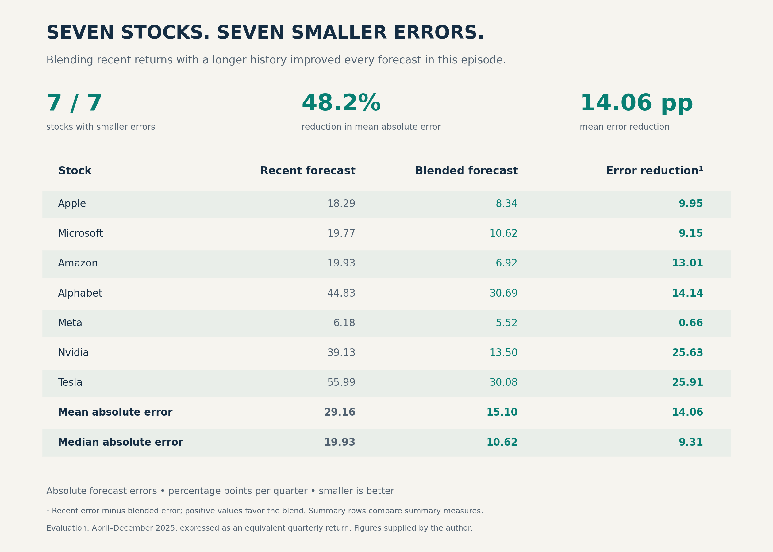
The image at the beginning of this article presents the individual errors and summary results. The blended forecast had the smaller absolute error for every stock. Its advantage ranged from 0.66 percentage points for Meta to 25.91 percentage points for Tesla.
Across the seven firms, the mean absolute error fell from 29.16 to 15.10 percentage points, a reduction of approximately 48.2 percent. The median absolute error fell from 19.93 to 10.62 percentage points. Errors are measured in percentage points per quarter; smaller values indicate more accurate forecasts.
Apple illustrates the calculation. Its quarterly equivalent return during 2023–2024 was 8.69 percent, while its first-quarter 2025 return was −11.20 percent. Averaging those observations produced a forecast of approximately −1.25 percent. Its subsequent April–December return was equivalent to 7.09 percent per quarter. The blend therefore missed by 8.34 percentage points, compared with 18.29 percentage points for the recent-performance forecast.
The blend was better, but it was hardly a precise forecast. It predicted negative returns for five of the seven firms, while all seven subsequently rose.
What can we learn?
The result shows how costly it can be to extrapolate a short period of performance. All seven stocks declined during the first quarter of 2025. Their earlier gains moderated those negative forecasts, bringing them closer to the subsequent positive returns.
However, better performance in this comparison does not establish that equal weighting is optimal. The 50–50 weight was specified for the exercise rather than estimated. Nor does the comparison show whether blending was better than using the historical quarterly rate alone. That is a natural additional benchmark.
The experiment also does not establish a profitable trading rule. Forecast accuracy and investment performance are different questions. Turning these forecasts into a strategy would require decisions about portfolio weights, holding periods, risk, and trading costs.
Conclusion
This exercise offers a modest illustration of an idea that made Efron and Morris’s work so memorable to me: an extreme recent observation need not be the best guide to what comes next. Here, combining recent returns with a longer history improved forecasts for every stock examined.
The result is stark: seven stocks, seven improvements, and an almost halving of mean absolute error. A superstitious hitter who goes seven for seven might decide he should not even change his underwear. A researcher should enjoy the streak—and then test whether it continues.
This is only one episode involving a distinctive group of firms. The seven stocks experienced the same broad sequence of earlier gains, first-quarter losses, and subsequent recovery. Seven firms moving through one market episode do not provide seven independent tests of a general forecasting principle.
Survival also matters. These are the Magnificent Seven, and none of the firms failed during the evaluation period. An experiment involving smaller companies with a higher rate of failure could produce different results. Such a study would need to retain firms that failed or were delisted, including the losses investors experienced, rather than examine only the survivors.
Finally, this exercise uses each firm’s own historical returns. Efron and Morris’s distinctive contribution involved borrowing information across individuals. Testing whether information across firms improves these forecasts remains a separate research question.
Author’s note: The downloadable Excel appendix below the paywall contains the source prices, return calculations, forecasting formulas, individual errors, summary measures, and detailed methodology—allowing you to examine and reproduce the experiment. It is a great buy for readers interested in exploring the numbers, and an annual subscription to Economic Memos costs only $30, including access to this appendix and my other paid content.
The Data Appendix in an Excel file.
